Linking correlation to probability - The binary way

Is there a link between the linear correlation coefficient and conditional probability?

One day, after observing that the correlation between two zero mean variables was 0.3, someone asked whether this meant that if one variable was positive the probability of the other one being positive is 0.3 too.

The short answer is no, but it’s not that straightforward to explain why; is it that that’s not the right figure or that correlation cannot be interpreted in such a way? The questioner had an interesting intuition, after all, if correlation measures linear dependency of random variables, shouldn’t there be some connection to conditional probabilities (i.e., to the probability of one variable matching the other’s variable variation) at some point?

Binary transformation

The first thing to notice is that the way the question is posed the interest is centered on binary outcomes (positive vs negative) while we often measure correlation for continuous variables (as in fact was the case in the aforementioned presentation).

Hence, the first step in bridging the gap between correlation and probability as framed in this case is to make our continuous variables binary. We call $A$ and $B$ the events in which the original continuous variables $X$ and $Y$ are above their respective thresholds $\theta_x$ and $\theta_y$ and we define the indicator (binary) variables $I_A$ and $I_B$ as:

$$I_A = \mathbb{1}_{X>\theta_x}, \\ I_B = \mathbb{1}_{Y>\theta_y}.$$

Of course in some cases our variables might be binary to begin with and we can ignore this step.

Correlation and its constituents

Now let’s recall the definition of correlation, which is none other than the covariance (how two variables vary together), normalized by each variable’s variance, so as to have a scale-independent output, always in the [-1, 1] interval.

$$\text{Corr}(I_A, I_B) = \frac{\text{Cov}(I_A, I_B)}{\sqrt{\text{Var}(I_A)\text{Var}(I_B)}}.$$

Since the goal of this investigation is to bridge correlation with probability, in the following lines we are going to express the variance and covariance in terms of the probabilities of $A$ and $B$.

Covariance

Let’s leave the variances for a moment and focus on covariance.

$$\text{Cov}(I_A, I_B) = \mathbb{E}[I_A I_B] - \mathbb{E}[I_A]\mathbb{E}[I_B]$$

Note that the product $I_A I_B$ will be 0 if either variable is 0 and 1 in the intersection $A \cap B$, hence its expected value is the probability of the intersection:

$$\mathbb{E}[I_A I_B] = P(A \cap B).$$

For the other expectations we simply have:

$$\mathbb{E}[I_A] = P(A), \quad \mathbb{E}[I_B] = P(B),$$

which we can now substitute in the original expression:

$$\text{Cov}(I_A, I_B) = P(A \cap B) - P(A)P(B).$$

We can also rearrange the expression of the intersection conditioning on one of the variables, let’s say $A$, which allows us to take out $P(A)$ as a common term:

$$\begin{aligned} \text{Cov}(I_A, I_B) & = P(A \cap B) - P(A)P(B) \\ & = P(B|A) P(A) - P(A)P(B) \\ & = [P(B|A) - P(B)] P(A). \end{aligned}$$

Analogously, we can decompose $P(B)$ conditioning on $A$: $P(B) = P(B|A)P(A) + P(B|A^c)P(A^c)$, where $c$ represents the complementary outcome, i.e., $P(A) = 1 - P(A^c)$.

$$\begin{aligned} \text{Cov}(I_A, I_B) & = [P(B|A) - P(B)] P(A) \\ & = [P(B|A) - P(B|A)P(A) - P(B|A^c)P(A^c)] P(A). \end{aligned}$$

We replace $P(A)$ in the second term in the brackets by $1-P(A^c)$ so as to make some cancellations:

$$\begin{aligned} \text{Cov}(I_A, I_B) & = [P(B|A) - P(B|A)[1 - P(A^c)] - P(B|A^c)P(A^c)] P(A) \\ & = [P(B|A)- P(B|A^c)] P(A^c)P(A). \end{aligned}$$

This will suffice, now let’s get back to variances.

Variance

Variance is nothing but the covariance of a variable with itself:

$$\begin{aligned} \text{Var}(I_A) & = \text{Cov}(I_A, I_A) \\ & = \mathbb{E}[I_A^2]- \mathbb{E}[I_A]^2. \end{aligned}$$

Since $I_A$ can only take 0 or 1 values, squaring it makes no difference:

$$\begin{aligned} \text{Var}(I_A) & = \mathbb{E}[I_A]- \mathbb{E}[I_A]^2 \\ & = P(A) - P(A)^2 = P(A) [1 - P(A)] = P(A)P(A^c). \end{aligned}$$

Obviously the same applies to any other binary variable like $I_B$.

Bringing all together

Now we have all the ingredients to get an expression of correlation that is linked to conditional probabilities in the way it was conceived in the starting question. Let’s start by substituting our previous results in the definition of correlation:

$$\begin{aligned} \text{Corr}(A,B) & = \frac{\text{Cov}(A,B)}{\sqrt{\text{Var}(A)\text{Var}(B)}} \\ & = \frac{[P(B|A)- P(B|A^c)] P(A^c)P(A)}{\sqrt{P(A)P(A^c)P(B)P(B^c)}} \end{aligned}$$

A little bit of rearrangement yields a cleaner expression:

$$\text{Corr}(A,B) = [P(B|A)- P(B|A^c)] \sqrt{\frac{P(A^c)P(A)}{P(B)P(B^c)}}.$$

So correlation is linked to the difference in the probability of $Y$ being positive (here we are assuming $\theta_x = \theta_y = 0$ as in the initial statement of the problem) when $X$ is positive versus negative. Notice how negative correlation implies that positive values of $Y$ are less likely when $X$ is positive as expected. The square root is always positive and can be understood as a scaling factor that ensures correlation stays within its expected boundaries.

Easing interpretability

We can make a last simplifying assumption to get rid of the scaling factor which is slightly hindering interpretability. If we place the binarizing thresholds ($\theta_x$ and $\theta_y$) in the median (or equivalently the mean, when the variable is symmetric), we will have $P(A)=P(A^c)=P(B)=P(B^c) = 0.5$ and hence:

$$\text{Corr}(I_A, I_B) = P(B|A) - P(B|A^c).$$

Since, $P(B) = P(B|A)P(A) + P(B|A^c)P(A^c) = 0.5 \medspace \Rightarrow \medspace P(B|A^c) = 1 - P(B|A)$, we can take it a little bit further:

$$\text{Corr}(I_A, I_B) = 2P(B|A) - 1.$$

When we are given a correlation and want to convert it to conditional probability we would use the following alternative arrangement:

$$P(B|A) = 0.5 + \frac{\text{Corr}(I_A, I_B)}{2}.$$

Since 0.5 is the marginal probability of $B$, the above expression means that knowing the event $A$ has happened, increases the probability of $B$ by half the correlation between the indicator variables.

We can make a handful of checks to see everything seems right. As expected, when the correlation is 0, we have $P(B|A) = 0.5$, as the two variables are independent, so knowing $A$ changes nothing. If it’s 1, $P(B|A) = 1$, as $A$ and $B$ share the same probability space. Conversely, if it’s -1, $P(B|A)=0$.

Answering the initial question

Going back to our initial example (and including the assumptions we’ve made along the way), if after binarizing we got a correlation of, let’s say, 0.2, that would mean that the probability of $Y$ being positive when $X$ is positive is 0.5 + 0.2/2 = 0.6.

Quick comment on the continuous approach

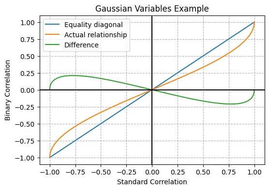
It’s possible to derive directly from a continuous bivariate distribution the conditional probability without recalculating correlation for the indicator variables. This path is however more analytically complex and so it will be left for another time. To get an idea on how results may differ, in the most common case of the normal bivariate distribution, we would have:

$$P(B|A) = 0.5 + \frac{\arcsin \text{Corr}(X, Y)}{\pi}.$$

Identifying terms with our previous expression we can see that:

$$\text{Corr}(I_A, I_B) = \frac{2}{\pi} \arcsin \text{Corr}(X, Y).$$

As a side note, the value $\text{Corr}(I_A, I_B) = 0.2$ we used in the previous section comes precisely from applying this equation to our original correlation of 0.3. Since $\arcsin 1 = \frac{\pi}{2}, \medspace \text{Corr}(X, Y) = 1 \medspace \Rightarrow \medspace \text{Corr}(I_A, I_B) = 1$, which seems natural. Equality holds at 0 too, and for the values in between the binary correlation is slightly smaller in magnitude (absolute value), reaching a maximum deviation of less than 0.25 at around 0.75, as can be seen in the plot below.