The Bayesian way to the raven paradox (Addendum): parameter updating

In our previous discussion of Bayesian inference for the raven paradox we have overlooked an interesting feature that’s worth coming back to.

Since the paradox is about contrasting the evidence in favor of “all ravens are black” ($B$) vs “not all ravens are black” ($B^c$) we haven’t paid much attention to the parameter/s we used to define $B^c$, specifically the number of black ravens assuming not all of them are black ($n_b|B^c$).

Recall this parameter could take many values so we assigned probabilitites to each of them through a probability distribution. We considered two possibilities, the simplest was a uniform distribution, meaning any number of black ravens (from $n_b=0$ to $n_b=n_r-1$) had the same probability: $P(n_b=k |B^c) = \frac{1}{n_r}$ (where $n_r$ is the number of ravens, which we set to a thousand $n_r=1000$). We then saw this led to a model that was heavily biased towards the existence of black ravens and considered a more balanced version that assigned higher probability to black ravens being few: $P(n_b=k | B^c) \propto \frac{1}{k}$.

The interesting feature we wanted to bring attention to is that as we update the probabilities of $B$ we are also implicitly updating the probabilities of $n_b|B^c$, which is also the reason we called the distributions above “priors”. In many applications these probabilities are as relevant as those of the hypothesis $B$ and $B^c$; for instance for predictive purposes, or even more so, if for some reason we are already commited to one hypothesis.

1. Parameter updating

So how does this work? It’s pretty much the same story as before, straight application of Bayes’ rule, but now, rather than $P(B | b_1, b_2, ..., b_n)$ we are after $P(n_b | b_1, b_2, ..., b_n, B^c)$:

$$\begin{equation*}\tag{1} P(n_b | b_1, b_2, ..., b_n, B^c) = \frac{P(b_1, b_2, ..., b_n | n_b, B^c)P(n_b | B^c)}{P(b_1, b_2, ..., b_n | B^c)}. \end{equation*}$$

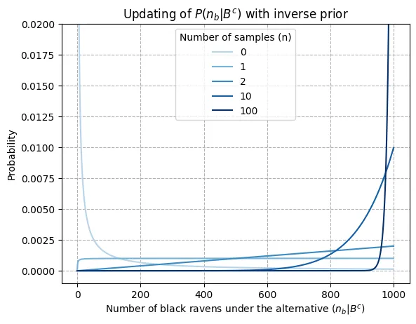
Note that we know all the terms on the right hand side from our previous calculations. Thus we can already take a look at how the probability for each number of black ravens under the alternative (“not all ravens are black”) is updated. In the graph below, we plot $P(n_b| b_1, b_2, ..., b_n, B^c)$ for different values of $n$ (i.e., black ravens observed), where $n=0$ corresponds to the prior probability, that is: $P(n_b | B^c)$.

Without observations (lightest blue), the inverse prior places much higher probabilities on there being a small number of black ravens. One observation is enough to turn this probability distribution flat (uniform)¹. An additional observation tilts the curve towards the right, placing higher probabilities on the number of black ravens being large. Already with 10 observations the probability of there being less than 600 black ravens is practically 0, and this figure rises to 950 for 100 observations².

So for $n=100$ if not all ravens where black (which at that point is already considered rather unlikely according to our previous posts) at least 950 are almost guaranteed to be so. As mentioned earlier, this kind of information can be used for predictive purposes, for instance if we want to get an estimate on the probability that the next raven we see will be black.

2. Different priors

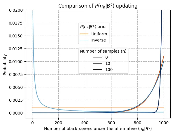
Now along with the inverse prior on $n_b$ we also considered a uniform one, how do their updates differ? In the comparison below, the contrast between the priors (lightest colors) is clear, but as data comes in the distributions converge quickly, being almost equal for $n=10$ and completely superimposed for $n=100$. This makes sense as it’s a general feature of Bayesian inference that priors are most relevant when evidence is limited, but as the sample size increases data imposes itself and priors are forgotten, which is a desirable behavior as well.

A point could be made here that the fact that the inverse prior after the first update becomes an almost uniform distribution sets up the two configurations for convergence. In other words, the uniform prior is a distribution that is kind of one step ahead of the inverse, so as more samples come in and the additional information brought by the next sample becomes smaller, the update per step gets reduced and the difference between one step and the next vanishes, leading to the overlap of the two distributions. Still, any other configuration would have lead to the same convergence (with one notable exception, assigning 0 probability to any $n_b$ value prevents making updates), although perhaps more slowly if the starting distributions are further apart³.

2.1 Iterative process and implicit updating

Reflecting on the previous posts after reading the above the following question may come to mind: why didn’t we update $P(n_b|B^c)$ in our calculations there? Perhaps the most intuitive approach at this point would have been to run an iterative process in which at each step $k$, both $P(B)$ and $P(n_b)$ are obtained incrementally from the previous iteration through the Bayes rule (recalling $P(b_k | B, b_1, b_2, ..., b_{k-1}) = 1$):

$$\begin{align*} &P(B | b_1, b_2, ..., b_k) = \frac{P(b_k | B, b_1, b_2, ..., b_{k-1})P(B | b_1, b_2, ..., b_{k-1})}{P(b_k | b_1, b_2, ..., b_{k-1})} = \\ & \qquad \qquad \qquad \qquad \enspace \frac{P(B | b_1, b_2, ..., b_{k-1})}{P(b_k | b_1, b_2, ..., b_{k-1})}, \tag{2} \\[5mm] &P(n_b | b_1, b_2, ..., b_k, B^c) = \frac{P(b_k | n_b, B^c)P(n_b | b_1, b_2, ..., b_{k-1}, B^c)}{P(b_k, B^c)}. \tag{3} \end{align*}$$

Equation (2) looks quite nice due to symmetry and it’s also rather intuitive. The probability of $B$ in each step equals that of the previous step divided by the predictive probability of seeing another black raven. The latter has to be a number less than 1, therefore making the probability of $B$ incrementally larger. The smaller the predictive probability of seeing another black raven —that is, the more probability $B^c$ has placed on the number of black ravens $n_b$ being small— the stronger the updates. This also serves to highlight the connection between (2) and (3). Renaming the probability of $B$ and $n_b$ after seeing $k$ samples as $P(B^k)$ and $P(n_b^k)$ respectively, we could describe the process at a high level where dependencies are made explicit as follows:

$$\begin{align*} \begin{cases} P(B^k) = f\left( P(B^{k-1}), P(n_b^{k-1}) \right), \tag{4} \\[2mm] P(n_b^k) = f\left( P(n_b^{k-1}) \right). \end{cases} \end{align*}$$

Again, the fact that in this iterative approach we are updating $P(n_b)$ each time unlike in our previous batch approach can make it look like the calculations are fundamentally different and could end up getting different results. Fortunately we don’t; were this to happen, it would reveal some failure in the batch approach described in our earlier posts to fully incorporate all the information provided⁴.

Actually this cannot be the case⁵ because we have been doing the same thing all along, namely: applying Bayes rule. If there’s to be any confusion at all it’s because in the batch approach some intermediate updates are in disguise, whereas the iterative approach is more explicit.

2.2 Batch approach unravelled

Let’s take a look at a decomposition of the batch approach that makes this more salient. We will consider the case of two observations $n=2$ as for any higher number one can get an analogous result by induction (in the same way that knowing how to sum two numbers, $x+y$, allows you to sum three, $x+y+z$, by first summing two of them, $x+y=t$, and then summing the result with the remaining third, $t+z$). Recall that

$$\begin{equation*}\tag{5} P(B | b_1, b_2) = \frac{P(B)}{P(B) + (1 - P(B))P(b_1, b_2 | B^c)}, \end{equation*}$$

and as $P(B)$ is a prior probability we specify, it all boils down to the term $P(b_1, b_2 | B^c)$. Previously we calculated this term directly as

$$\begin{equation*}\tag{6} P(b_1, b_2 | B^c) = \sum_{k=0}^{n_r-1} P(b_1, b_2 | n_b=k) P(n_b=k | B^c). \end{equation*}$$

However, we can also apply the chain rule to find how the probabilitites of $P(n_b)$ are being implicitly updated:

$$\begin{equation*}\tag{7} P(b_1, b_2 | B^c) = P(b_1| B^c) P(b_2 | b_1, B^c), \end{equation*}$$

where each term is defined as follows:

$$\begin{cases} P(b_1| B^c) &= \sum_{k=0}^{n_r-1} P(b_1 | n_b=k) P(n_b=k | B^c), \\ P(b_2 | b_1, B^c) &= \sum_{k=0}^{n_r-1} P(b_2 | n_b=k) P(n_b=k | b_1, B^c). \tag{8} \end{cases}$$

Note that for the first term the prior distribution is used $P(n_b | B^c)$ however for the second term this is replaced by an update that considers the previous sample $P(n_b | b_1, B^c)$. Thus, the probability distribution of $P(n_b)$ is indeed being updated but in an implicit fashion that it’s not clearly visible at first.

3. Wrapping up

We have seen that Bayes rule serves not only to update probabilities on different hypothesis being true as data comes in, but also to update how this hypotheses look like. Although it’s here that this second update has been made explicit, it was already being inadvertedly carried out when performing the first. In particular, as more black ravens are identified not only the prospect of all of them becomes more likely, but also if they were not, it becomes increasingly certain that the number of black ravens should be considerably large. Probably not the most astounding conclusions and gladly so, because otherwise we could be in trouble. However the key is not in the results, but in the tools that allow for a proper formalization and quantification of inference which can be applied to real life problems.

Footnotes

1. You may have seen it’s not entirely uniform on the left hand side. This is because the probability of there being no black ravens is zero, $P(n_b=0|b_1, B^c) = 0$, for we have just seen one. ↩

2. Recall that it’s indeed extremely unlikely to see 10 consecutive black ravens if less than 600 hundred of them are black. A quick upper bound can be obtained via: $P(b_1, b_2, ..., b_{10} | n_b=600) \leq (600/1000)^{10} \simeq 0.006$. Contrast this with $P(b_1, b_2, ..., b_{10} | n_b=900) \leq (900/1000)^{10} \simeq 0.35$. ↩

3. What would further apart mean here? We have intuitively used as a measure of distance the number of steps away from each other. This distance would be increased if we replaced the uniform by a distribution closer (now “closer” in the common sense of being nearby in the graph) to the limiting distribution (i.e., heavily tilted towards the right) and the inverse by a distribution that’s on the other end (even more tilted towards the left than the inverse already is). That being said, “steps away from each other” is not the best measure of distance as there are many different paths to convergence, but it’s useful enough for our discussion. ↩

4. We are doubting the validity of the batch approach because when we update iteratively we are guaranteeing at each step that we make maximal use of the available information. ↩

5. Well it can, but due to numerical errors and that’s a different issue which is not a matter of concern for our purposes. In such events, generally the batch approach will yield more accurate results as it’s reducing the number of operations which are ultimately the source of errors. ↩