The Bayesian way to the raven paradox (II): contrapositive and conclusion

So coming back from our earlier post we already had the following model (based on Bayes’ rule) for assessing the proposition “all ravens are black” (which we named $B$):

$$\begin{align*} P(B& | b_1, b_2, ..., b_n) = \frac{P(B)}{P(B) + P(b_1, b_2, ..., b_n | B^c)(1 - P(B))} = \\ & \frac{P(B)}{P(B) + (1 - P(B)) \sum_{k=0}^{n_r-1} P(n_b = k | B^c) \prod_{i=0}^{n-1} \left( \frac{k-i}{n_r-i} \right)}. \tag{1} \end{align*}$$

Recall that $b_i$ were events of seeing each one distinct black raven (somehow randomly sampled from the set of all ravens). We also named $n$ the total number of samples, $n_r$ the total number of ravens and $n_b$ the number of black ravens, which only made sense to specifiy under the alternative hypothesis $B^c$: “not all ravens are black”.

1. A model for the contrapositive

Given the degree of analogy between our original proposition and the contrapositive, building a model for the latter practically amounts to renaming variables in the former’s model. To highlight the similarities, our renaming will be limited to adding a “hat” ($x \rightarrow \hat{x}$) on top of the original symbols. So we have:

• $\hat{B}$: the proposition “all non-black things are non-ravens”.
• $\hat{b}_i$: an instance of seeing a non-black non-raven thing.
• $\hat{n}$: the sample size.
• $\hat{n}_r$: the total number of non-black things.
• $\hat{B}^c$: the proposition “not all non-black things are non-ravens” (triple negation!).
• $\hat{n}_{\hat{b}}$: the number of non-black non-raven things (generally it only makes sense to specify this number under the alternative, which can be expressed more explicitly as $\hat{n}_{\hat{b}} | \hat{B}^c$).

This is going to be quite quick. Note that all the propositions and arguments we’ve made in the previous post are anologous if we just replace the old variables ($x$) with the new ones ($\hat{x}$), and so the result should be the same (feel free to review these steps as it is a nice exercise too). The only thing that requires more careful thought is defining $P(\hat{n}_b | \hat{B}^c)$ but this can be worked out by realising that $\hat{n}_b = n_b + \hat{n}_r - n_r$, so $P(n_b=k | B^c) = P(\hat{n}_b = k + \hat{n}_r - n_r | \hat{B}^c)$, given that $B^c$ and $\hat{B}^c$ are equivalent.

$$\begin{align*} &P(\hat{B} | \hat{b}_1, \hat{b}_2, ..., \hat{b}_{\hat{n}}) = \frac{P(\hat{B})}{P(\hat{B}) + P(\hat{b}_1, \hat{b}_2, ..., \hat{b}_{\hat{n}} | \hat{B}^c)(1 - P(\hat{B}))} = \\ & \quad \frac{P(\hat{B})}{P(\hat{B}) + (1 - P(\hat{B})) \sum_{m=\hat{n}_r - n_r}^{\hat{n}_r-1} P(\hat{n}_b = m | \hat{B}^c) \prod_{j=0}^{\hat{n}-1} \left( \frac{m-j}{\hat{n}_r-j} \right)}. \tag{2} \end{align*}$$

Note that since $B$ and $\hat{B}$ are logically equivalent we have $P(B) = P(\hat{B})$. Also as stated we have $P(n_b=k | B^c) = P(\hat{n}_b = k + \hat{n}_r - n_r | \hat{B}^c)$. We can use these equalitites to subsitute in (2) and make the differences between the model from the previous post and the contrapositive more explicit:

$$\begin{align*} &P(B | \hat{b}_1, \hat{b}_2, ..., \hat{b}_{\hat{n}}) = \\ & \quad \frac{P(B)}{P(B) + (1 - P(B)) \sum_{k=0}^{n_r-1} P(n_b=k | B^c) \prod_{i=0}^{\hat{n}-1} \left( \frac{\hat{n}_r - n_r + k - i}{\hat{n}_r-i} \right)}. \tag{3} \end{align*}$$

There we have it. Looking at this equation we see that with respect to the experiments in the previous post (i.e., with respect to (1)), the only new parameter that we have to set is $\hat{n}_r$, the number of non-black things (technically we have to consider $\hat{n}$ too, but soon it will become clear why we don’t think of it as an additional parameter).

Back to the paradox

Now a reasonable question to make is whether the result we get via the contrapositive is the same as the one from attempting to prove the original proposition (for a choice of $n$ and $\hat{n}$ that is aligned with our initial discussion):

$$P(B | b_1, b_2, ..., b_n) \stackrel{?}{=} P(\hat{B} | \hat{b}_1, \hat{b}_2, ..., \hat{b}_{\hat{n}}).$$

Which in our model boils down to:

$$\begin{align*} &\sum_{k=0}^{n_r-1} P(n_b=k | B^c) \prod_{i=0}^{n-1} \left( \frac{k-i}{n_r-i} \right) \stackrel{?}{=} \\ &\sum_{k=0}^{n_r-1} P(n_b=k | B^c) \prod_{j=0}^{\hat{n}-1} \left( \frac{\hat{n}_r - n_r + k-j}{\hat{n}_r-j} \right). \end{align*}$$

One way to reformulate this question would be to ask whether there’s the same amount of information in ${b_1, b_2, ..., b_n}$ as in ${\hat{b}_1, \hat{b}_2, ..., \hat{b}_{\hat{n}}}$. Note that the raven paradox is not about these quantities being equal (in fact we’ll see they’re not) but related in some vague sense. Still, we can see that the prospect of equality is not that absurd.

First, on both sides of the “equation” we have a sum with the same number of terms so it’s all about the products within. These are products of values slightly less than 1 (it’s only because they are extremely close to 1 that it’s possible to have large products without the result shrinking to 0), so the result decreases both as more terms are added to the product and as these terms become smaller. It will become clear soon when we specify the value of $\hat{n}$ that the right hand side will have many more terms (as the number of black things is much greater than that of ravens), but this is compensated by the fact that they are also closer to 1 (again precisely because $n_r \ll \hat{n}_r$) hence shrinking slower. In fact we will see that this compensation works quite well most of the time, but let’s not get ahead of ourselves.

2. Final comparison: original vs contrapositive.

We can now reproduce an experiment similar to that of the previous post and see how the two approaches that make up the raven paradox compare. We will consider a population of a thousand ravens ($n_r=1000$) and a number of black things of a million ($\hat{n}_r = 10^6$). Clearly these data are not realistic but they work perfectly fine for the purpose of our demonstrations. As before, we consider two different sets of priors to characterize the alternative $B^c$. Finally, the sample size is not expressed in absolute terms (number of samples) but in relative terms (fraction of the total population) so as to make the two approaches for proving $B$ the most equivalent possible (following our initial discussion). Thus we call $f$ the sampling fraction: $f = \frac{n}{n_r} = \frac{\hat{n}}{\hat{n}_r}$, and then by setting values of $f$ we get the number of samples in each case via: $n = fn_r$ and $\hat{n} = f\hat{n}_r$¹.

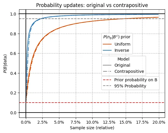
We can see below the comparison between the probability updates we get using the original model (i.e., looking for black ravens) versus using the contrapositive model (i.e., looking for non-black non-raven things). For the two choices of priors on $n_b$ (see the previous post for an explanation on these²) both approaches seem to result in very similar probability updates.

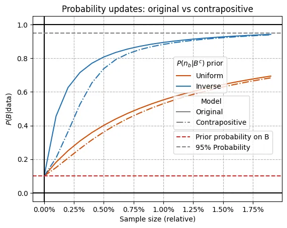
If we zoom a little bit on the smaller sample sizes where the difference is greatest (see plot below), we find that the contrapositive model results in slightly slower updates, needing at most something less than 0.25% (more generally less than 0.10%) additional samples to reach the same degree of belief in $B$.

So evidence for the contrapositive turns out to be less informative, how so? Well, if we’ve seen non-black non-raven things, it could be that that’s because ravens are black, or just because no raven happened to be included in the sample. The possibility of failing to sample ravens seems more relevant when the population size of the non-black things is higher compared to that of ravens. Now this is only impactful for small sample sizes because at some point, no matter how small the raven population is, you are almost guaranteed to pick one if they are non-black.

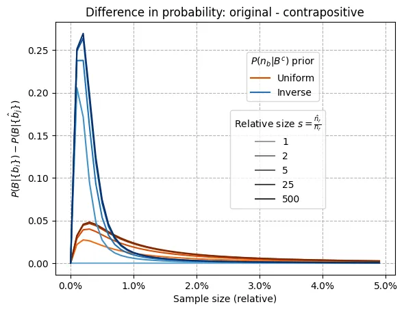
Let’s take a look at the differences between the probability updates for the original and the contrapositive model as shown in the plot below. To assess how the relatively small population of black ravens affects the deviations we consider different sizes expressed as a ratio $s = \frac{\hat{n}_r}{n_r}$. For $s=1$, there are as many non-black things as ravens, so the models are equivalent and there should be no differences (the light orange line is not discernible because it’s completely covered by the light blue line as expected).

As $s$ grows larger (there are more non-black things than ravens), contrapositive samples become less informative. Interestingly, most of the difference is observed when doubling the relative size ($s=25$ and $s=1000$ are practically on top of each other, so fairly quickly the deviation reaches some sort of saturation). Also, notice that differences can be rather high, up to 0.25 (for the uniform model that is, which is understandable since it has very strong updates at the beginning) although for a very limited range of sample sizes, and beyond 2% they stay below 0.01.

Why is already a value of $s=2$ enough to create a significant gap? A key aspect here is that when seeing $n$ black ravens we can automatically set to 0 the probability of any value of $n_b$ smaller than $n$, which allows for strong updates. When $\hat{n}_r = n_r$ we can do the same after seeing $\hat{n}$ non-black non-raven things (if there are as many non-black things as ravens, seeing one non-black non-raven thing already means that at most 999 ravens are non-black hence at least one raven is black) but we quickly lose this ability as $\hat{n_r}$ becomes larger. Although these probabilities are already quite small to begin with, we have already seen that the difference between quite small and zero can be rather significant.

It’s important to bear in mind that although in the big picture (i.e., first plot) the two approaches seem to yield very similar results, we have been equating relative sample sizes all along. This means that since the population of the contrapositive is much larger, we also need many more samples, and in that way it can be considered a less efficient process of inference.

3. Back to the paradox and conclusion

Besides the fact that the contrapositive route is a slower path towards strenghening our belief in all ravens being black, the truth is that seeing a non-black non-raven thing does help³. Given the limited magnitude of the deviations in probability with respect to the original, we can confirm that the solution proposed initially remarking the importance of equating relative sample sizes was rather accurate.

The paradox appears as such because, in real life, equating relative sample sizes is not even a possibility due to the ridiculuous amount of non-black things that exist. Considering that there are 16 million ravens ($10^7$ onwards) and we’ll (very very very roughly) estimate between $10^{20}$ and $10^{30}$ non-black things ($10^{25}$ onwards), we have that for every black raven we see, we should see $\frac{10^{25}}{10^7} = 10^{18}$ non-black non-raven things. To give an idea, if we count two distinct non-black non-raven things per second, that amounts to $2 \cdot 60^2 \cdot 24 \cdot 365 \cdot 100 < 10^{10}$ if we kept every second of a 100 years on the lookout.

To recap, our initial point was that at its core the raven paradox is born out of language vagueness which concealed the significance of the quantitative differences between the two seemingly equivalent ways to proof that all ravens are black. By introducing a more formal analysis, it has become clear that the paradox is not such, but just an apparently counterintuitive result that becomes more digestible as quantities are made precise.

This formalization of inference also helps reveal some nuances regarding the ways in which we can leverage data to assess our hypotheses (and make predictions), such as the informative power of randomness and the inefficiency (but also potential utility) of contrapositive statements. Of course, here we have relied in some simplifications, since we weren’t really that concerned about the color of ravens. In real life applications this process can get quite involved but hardly ever not worth the effort, as it is difficult to overestimate the benefits that striving for systematicity and precision bring to decision theory.

If you are in for a little bit more of Bayesian discussion you may want to click here.

Footnotes

1. This is the reason why we didn’t consider $\hat{n}$ an additional parameter, as it’s determined by $f$ which was already implicitly set (although we didn’t point it out at that time) for the original model. ↩

2. As a brief summary, these priors represent $P(n_b|B^c)$, that is, the probability of $n_b$ ravens being black under the hypothesis “not all ravens are black” ($B^c$). “Uniform” means any number of black ravens being equally likely whereas “inverse” means probability being inverse to the number of black ravens (i.e., it’s more likely that black ravens are few). ↩

3. This means that the contrapositive can be used in those cases where testing the original proposition is more cumbersome or not even possible. For instance, considering the famous WWII plane reinforcement case, a hypothesis of the kind “planes that are hit in this area do not return” is hard to assess as presumably there are no samples to work with (i.e. no returning planes); however, the contrapositive “planes that return have not been hit in this area” does allow for the gathering of data to back it up. ↩