Application of mass conservation principle in a conic bottle

We spaniards are great olive oil consumers.

One day, at home, I filled up the olive oil bottle and then cooked with it.

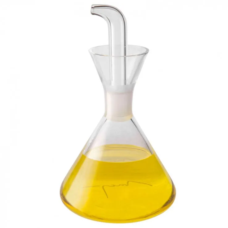
After the meal, jokingly, my girlfriend pointed out how much the olive oil level had decreased. I didn’t remember using that much oil, but she was right: the level of the liquid had decreased a lot since the very recent refill.

So it got me wondering: did I consume that much oil without realising it? Or is there something else going on? I decided to investigate the matter in more formal terms.

Brief Foreword

We will follow Polya’s problem solving method.

1. Understanding the problem: define variables, unknowns, relationships between them, and the actual question we want to address.
2. Devise a plan: which equations are we going to use? In what order are we going to solve them?
3. Carry out the plan: solve the equations, get as far as we can looking for a closed-form solution; push to the limits the need for numerical methods, i.e., what is the smallest problem we cannot solve analytically?
4. Look back and reflect.

As a closing remark, this is a divulgative post. The experienced reader will find it is approached in a very general way, in spite of the simplicity of the problem. This will allow for great simplifications early on. Our goal is to show clearly how more complicated versions would be addressed. Hence, we will include many details in the derivations that would be usually skipped.

Understanding the problem

As Polya very well points out in his book, the first step to solving a problem, and where we should spend most of the time, is understanding it.

Face up, the main fuzzy research question we want to answer is: does the liquid in a conical bottle empty faster at the start than at the end?

Intuitively, given the conic shape of the bottle, we can foresee that yes, indeed, the level drops faster at the beginning, but we want to formalize this intuition: more generally, given an outflow rate, what is the function of the liquid surface height as a function of time?

We will assume that the liquid is incompressible with density $\rho$, and that the bottle is a cone of height $H$ and base radius $R$.

What is the unknown?

The variable we are after is the height of the liquid as a function of time, $h(t)$. However, there is no straightforward way to solve for $h(t)$, i.e., there is no general law of fluid mechanics expressed in terms of this variable. We will need to play around to find a suitable equation to solve for $h(t)$.

A subtle simplification for the geometry

Truly, the actual motion of the problem is the liquid escaping the bottle through the cap at a constant rate when the bottle is turned to an angle.

However, it would be a bit messier to solve this geometrical setup, since we would have to account for a changing angle in time, and a non-trivial liquid volume shape.

Hence, on paper, we can simplify the problem to a bottle in a vertical position, and the liquid escaping the bottle at a constant rate through the cap through an imaginary thin tube that goes from the cap to the floor.

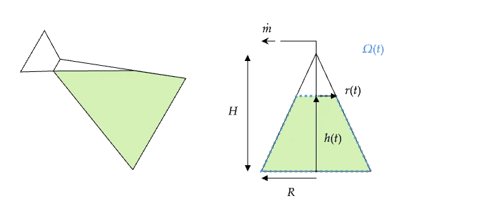
The thin tube is a mathematical trick to model the outflow of the liquid, we will consider it does not change significantly its dynamics or volume.

This problem has a gentler geometry and is equivalent to the original problem for the purpose of the research question.

Control volume

Now that we have cleared out the geometrical layout, it is customary in fluid mechanics to define a control volume. The control volume is the region in space that we choose to study the dynamics of the fluid.

For today’s problem, we are going to define the control volume as the moving volume of the liquid, $\Omega(t)$. The boundary is $\partial\Omega(t)$, and it has four constituents: the bottom of the bottle, the lateral surface, the liquid surface at the top (which is a moving boundary) and the cap of the bottle,

$$\partial\Omega(t) = \partial\Omega_{\text{bottom}} \cup \partial\Omega_{\text{lateral}} \cup \partial\Omega_{\text{top}}(t) \cup \partial\Omega_{\text{cap}}.$$

We have excluded the imaginary tube from the control volume, because it is not relevant for the mathematical model.

Volume to height relationship

We can express the volume of the liquid as a function of the height of the liquid in the bottle.

Given a truncated cone with base radius $R$, top radius $r(t)$, and height $h(t)$, the volume is

$$\begin{equation} \Omega(t) = \frac{\pi}{3} h(t) \left(R^2 + r(t)^2 + R \cdot r(t)\right). \end{equation}$$

This expression connects our variable of interest with a variable that is likely to appear in the equations we are going to use, bridging a bit further the gap towards an equation for $h(t)$.

However, it is still too raw, as it contains another unknown, the radius of the liquid surface $r(t)$. We need to further mess with the geometry to remove the radius of the liquid surface from the equation.

The middle section of the bottle has a truncated triangle. If we extend it to the top of the bottle, we get a congruent triangle. This is a very useful observation, because it allows us to relate the radius of the liquid surface with the height of the liquid in the bottle.

Hence, given the triangle with base $R$ and height $H$, the radius $r(t)$ and height $h(t)$ of the liquid surface are related by

$$\begin{align} \frac{R}{H} &= \frac{r(t)}{H - h(t)}, \\[5mm] r(t) &= R \cdot \left(1 - \frac{h(t)}{H}\right). \end{align}$$

At this point we find convenient to introduce the dimensionless variable $\hat{h}(t)$,

$$\begin{equation} \hat{h}(t) = \frac{h(t)}{H}, \end{equation}$$

to simplify the expression. It is customary to use dimensionless variables in fluid mechanics. They make equations more general and easier to handle (I like to introduce them as they come up in the derivations, it makes their choice more organic and suited for the problem details).

Hence, the radius $r(t)$ becomes

$$\begin{equation} r(t) = R \cdot \left(1 - \hat{h}(t)\right). \end{equation}$$

Plugging this into the volume of the liquid, we get

$$\begin{align} \Omega(t) &= \frac{\pi}{3} h(t) \left(R^2 + r(t)^2 + R \cdot r(t)\right), \\[5mm] \Omega(t) &= \frac{\pi}{3} H \hat{h}(t) \left(R^2 + R^2 (1 - \hat{h}(t))^2 + R^2 (1 - \hat{h}(t))\right), \\[5mm] \Omega(t) &= \frac{\pi}{3} H R^2 \cdot \hat{h}(t) \cdot \left(1 + (1 - \hat{h}(t))^2 + (1 - \hat{h}(t))\right). \end{align}$$

The inside of the parenthesis is a polynomial of degree 2, crying out to be expanded and simplified.

$$\begin{equation} \Omega(t) = \frac{\pi}{3} H R^2 \cdot \hat{h}(t) \cdot \left(3 - 3 \hat{h}(t) + \hat{h}(t)^2\right). \end{equation}$$

This is really good progress, and we have not even started (apparently) solving the problem yet!

I think this is what Polya meant when he said that understanding the problem is a task we should stay at for a long time. Because we are investing time and effort laying out the foundations, we are already getting a good grasp of the problem. This will make the rest of the derivations much smoother and clearer, reducing the chances of making mistakes.

In the same spirit in which we introduced the dimensionless variable $\hat{h}(t)$, we find a natural reference volume $\Omega_0 = \frac{\pi}{3} H R^2$ (the volume of the full untruncated cone, which showed up naturally in the derivations, how cool is that? These are usual hints that we are on the right track!).

So, we use this reference volume to make the expression for the volume dimensionless too,

$$\begin{align} \Omega(t) &= \Omega_0 \cdot \hat{\Omega}(t), \\[5mm] \hat{\Omega}(t) &= \hat{h}(t) \cdot \left(3 - 3 \hat{h}(t) + \hat{h}(t)^2\right). \end{align}$$

You can verify by yourself that $\hat{\Omega}(0) = 1$.

Just to be clear, the general laws of fluid mechanics are expressed in terms of the physical variables, but it is a good practice to have the dimensionless variables in mind and ready, to plug them in the equations when necessary.

What happens at the boundaries?

Later on, when we are “carrying out the plan”, we will have to account for the velocity of the liquid at the boundaries, and of the boundary itself.

To keep our procedure tidy, we will make some observations now.

At the solid surfaces of the bottle (bottom and lateral), the velocity of the liquid in the normal direction to the surface is zero (they are impermeable surfaces).

$$\begin{align} \left.(\mathbf{v - v_c}) \cdot \mathbf{n} \right|_{\partial\Omega_\text{bottom}} = \left.\mathbf{v} \cdot \mathbf{n} \right|_{\partial\Omega_\text{bottom}} &= \mathbf{0}, \\[5mm] \left.(\mathbf{v - v_c}) \cdot \mathbf{n} \right|_{\partial\Omega_\text{lateral}} = \left.\mathbf{v} \cdot \mathbf{n} \right|_{\partial\Omega_\text{lateral}} &= \mathbf{0}. \end{align}$$

At the top surface, even if at this point the velocity of the liquid is unknown, because we have chosen the control volume to be the liquid itself, we know it is equal to the velocity of the control volume, $\left(\left.\mathbf{v}_c\right|_{\partial\Omega_\text{upper surface}} = -\frac{\text{d}h(t)}{\text{d}t} \mathbf{j}\right)$, so the term $\mathbf{v - v_c}$ is zero at the upper surface,

$$\begin{equation} \left.(\mathbf{v - v_c})\right|_{\partial\Omega_\text{upper surface}} = \mathbf{0}. \end{equation}$$

Finally, through the cap of the bottle the liquid goes out. We ignore the shape of the velocity distribution, but we can assume that the integral of the velocity of the liquid through the cap is a constant,

$$\begin{equation} \int_{\partial \Omega_{\text{cap}}} \rho \ \mathbf{v} \cdot \mathbf{n} \ \text{d}\sigma = \dot{m}. \end{equation}$$

Devising a plan

All right, so far we have well identified the unknown, pushed to the detail the variables and the relationships between them.

We have reached a point where we can start to think about the nature of the model equations we are going to solve.

Equations for the model

Broadly speaking, when addressing fluid mechanics problems, there are three main equations we can use: the conservation of mass, momentum, and energy. Each of these can be cast in its integral or differential form.

Since we are not interested in the velocity distribution inside the liquid, nor the magnitude of the forces acting on the liquid, or any energy-related quantity; but rather the evolution of its volume, we are going to use the mass conservation principle in its integral form:

$$\begin{equation} \frac{\text{d}}{\text{d}t} \int_{\Omega(t)} \rho \text{d}\Omega + \int_{\partial \Omega(t)} \rho (\mathbf{v - v_c}) \cdot \mathbf{n} \text{d}\sigma = 0. \end{equation}$$

Despite the integrals, this equation is simply a first order ODE in time.

Keeping in mind the true nature of the equations we are facing is helpful to orient the algebraic maneuvers along the problem solving process; and to define properly the boundary and initial conditions.

Can we identify the unknown of this ODE? Since the density $\rho$ is constant in time, when derivations have settled, the unknown will be the volume of the liquid as a function of time, $\Omega(t)$ (look at the first summand!).

Hence, we are after an equation that relates the derivative of the volume of the liquid with time and any other terms that will depend on the boundary integrals.

$$\frac{\text{d}\Omega(t)}{\text{d}t} + \text{additional terms} = 0.$$

We cannot anticipate yet the exact terms that will appear in the equation, but hopefully we will be able to solve it analytically (I am fond of numerical methods, but they introduce an additionaly layer of complexity that I prefer to keep for the last resort).

Boundary conditions for the integrals

To obtain this ODE, we will have to expand the integrals to show explicitly the boundaries in which they apply, and equip them with the observations we made earlier about the behaviours at the walls and holes of the bottle.

$$\begin{align} \frac{\text{d}}{\text{d}t} \int_{\Omega(t)} \rho \text{d}\Omega + \int_{\partial\Omega_{\text{bottom}} \cup \partial\Omega_{\text{lateral}} \cup \partial\Omega_{\text{top}}(t) \cup \partial\Omega_{\text{cap}}} \rho (\mathbf{v - v_c}) \cdot \mathbf{n} \text{d}\sigma &= 0, \\[5mm] \int_{\partial \Omega_{\text{cap}}} \rho \ \mathbf{v} \cdot \mathbf{n} \ \text{d}\sigma &= \dot{m}, \\[5mm] \left.(\mathbf{v - v_c})\right|_{\partial\Omega_\text{top}(t)} &= \mathbf{0}, \\[5mm] \left.(\mathbf{v - v_c}) \cdot \mathbf{n} \right|_{\partial\Omega_\text{bottom}} = \left.\mathbf{v} \cdot \mathbf{n} \right|_{\partial\Omega_\text{bottom}} &= \mathbf{0}, \\[5mm] \left.(\mathbf{v - v_c}) \cdot \mathbf{n} \right|_{\partial\Omega_\text{lateral}} = \left.\mathbf{v} \cdot \mathbf{n} \right|_{\partial\Omega_\text{lateral}} &= \mathbf{0}. \end{align}$$

Initial condition for the ODE

Since we have a first order ODE in time, we need to provide an initial condition for the volume of the liquid at time $t=0$. We can use the expression for the volume of the liquid at time $t=0$,

$$\Omega(0) = \Omega_0,$$

as the initial condition for the ODE.

Catching our breath

A lot of details have been covered so far.

To keep focus, we present a summary of the mathematical model we are going to use to solve the problem. We have two equations to solve:

• a differential equation in time for the volume of the liquid $\Omega(t)$, (the specific terms involved in it are yet to be determined in the “Carrying out the plan” stage),
• an algebraic equation that relates the volume $\Omega(t)$ with the height of the liquid $h(t)$, (we have already found the expression for the volume as a function of the height).

We recall that some dimensionless expressions have been introduced, which will be of help to find a general solution that is not tied to specific values of the parameters.

$$\begin{align} \text{Geometrical relations} \nonumber \\[5mm] \hat{h}(t) = \frac{h(t)}{H}, \\[5mm] \Omega(t) = \Omega_0 \cdot \hat{\Omega}(t), \quad \text{s.t.} \quad \Omega_0 = \frac{\pi}{3} H R^2. \\[5mm] \text{(Algebraic equation) Volume and height} \nonumber \\[5mm] \hat{\Omega}(t) = \hat{h}(t) \cdot \left(3 - 3 \hat{h}(t) + \hat{h}(t)^2\right). \\[5mm] \text{(ODE) Mass conservation equation} \nonumber \\[5mm] \frac{\text{d}}{\text{d}t} \int_{\Omega(t)} \rho \text{d}\Omega + \int_{\partial\Omega_{\text{bottom}} \cup \partial\Omega_{\text{lateral}} \cup \partial\Omega_{\text{top}}(t) \cup \partial\Omega_{\text{cap}}} \rho (\mathbf{v - v_c}) \cdot \mathbf{n} \text{d}\sigma &= 0, \\[5mm] \int_{\partial \Omega_{\text{cap}}} \rho \ \mathbf{v} \cdot \mathbf{n} \ \text{d}\sigma &= \dot{m}, \\[5mm] \left.(\mathbf{v - v_c})\right|_{\partial\Omega_\text{top}(t)} &= \mathbf{0}, \\[5mm] \left.(\mathbf{v - v_c}) \cdot \mathbf{n} \right|_{\partial\Omega_\text{bottom}} = \left.\mathbf{v} \cdot \mathbf{n} \right|_{\partial\Omega_\text{bottom}} &= \mathbf{0}, \\[5mm] \left.(\mathbf{v - v_c}) \cdot \mathbf{n} \right|_{\partial\Omega_\text{lateral}} = \left.\mathbf{v} \cdot \mathbf{n} \right|_{\partial\Omega_\text{lateral}} &= \mathbf{0}, \\[5mm] \Omega(0) &= \Omega_0. \end{align}$$

This is the complete mathematical model: from the initial fuzzy question to the specific equations we are going to solve.

Drafting the expected derivation workflow

This is the last consideration to be done, perhaps a delicate point in the problem-solving process.

It is delicate because, while we plan, we must embrace the exploratory essence of problem-solving, acknowledging that the solution’s nature remains unknown until it’s reached.

We cannot anticipate every single step we are going to take from now on (e.g., unexpected algebraic tricks might be required when integrals are truly expanded), nor can we tell now where the derivations will take us.

However, despite this “algebraic uncertainty”, drafting the main steps ensures we maintain a sense of direction. When the dust settles from the derivations, we have a roadmap to guide us.

1. Identifying the ODE:
   • Expand the surface integral in the mass conservation equation.
   • Use the boundary conditions to simplify the terms as much as possible.
   • Cast the ODE in a dimensionless form.
2. Solving the ODE to obtain the volume in time.
3. Solving the algebraic equation to obtain the height of the liquid as a function of time.

At this point we cannot tell if we will be able to go all the way down without the need for numerical methods.

It could be the case that the ODE needs to be solved numerically, and thus the algebraic equation as well. Until we do not execute this plan, we cannot tell.

However, our systematic approach has given us a good grasp of the problem, and we are ready to push the analytical derivations as far as we can.

Carrying out the plan

Yeah! This is an exciting moment too! Finally we get our hands dirty and start solving the equations.

Identifying the ODE

We expand the surface integral in the mass conservation equation to account for the three boundaries of the control volume,

$$\begin{equation} \begin{split} \frac{\text{d}}{\text{d}t} \int_{\Omega(t)} \rho \text{d}\Omega &+ \int_{\partial \Omega_{\text{bottom}}} \rho \ \mathbf{v} \cdot \mathbf{n} \ \text{d}\sigma \\[5mm] &+ \int_{\partial \Omega_{\text{lateral}}} \rho \ \mathbf{v} \cdot \mathbf{n}\ \text{d}\sigma \\[5mm] &+ \int_{\partial \Omega_{\text{top}}} \rho \ (\mathbf{v - v_c}) \cdot \mathbf{n} \ \text{d}\sigma \\[5mm] &+ \int_{\partial \Omega_{\text{cap}}} \rho \ \mathbf{v} \cdot \mathbf{n} \ \text{d}\sigma = 0. \end{split} \end{equation}$$

Through application of the boundary conditions, most integrals simplify to zero, and the one that does not simplifies to a constant,

$$\begin{equation} \frac{\text{d}}{\text{d}t} \Omega(t) + \dot{m} = 0. \end{equation}$$

Impressive hey, one step iteration and we have already found the ODE!

Solving the ODE

The previous ODE is now equipped with the initial condition. Before jumping into solving it, we will make it dimensionless too (at this point it should be clear the importance of having the dimensionless variables ready),

$$\begin{align} \Omega(t) &= \Omega_0 \cdot \hat{\Omega}(t), \\[5mm] \frac{\text{d}}{\text{d}t} \Omega(t) + \dot{m} &= 0, \\[5mm] \Omega_0 \frac{\text{d}}{\text{d}t} \hat{\Omega}(t) + \dot{m} &= 0, \\[5mm] \frac{\text{d}}{\text{d}t} \hat{\Omega}(t) &= - \frac{\dot{m}}{\Omega_0}. \end{align}$$

Is the ODE now dimensionless? Not fully, time is still in the equation with its physical units. To see clearly how we should make it dimensionless, a possibility given this equation is to first move the time differential to the other side of the equation, with the constant term

$$\begin{align} \text{d} \hat{\Omega}(t) &= - \frac{\dot{m}}{\Omega_0} \text{d}t. \end{align}$$

If the left hand side is dimensionless, then the right hand side is dimensionless as well.

Hence, it is easier to make the right hand side dimensionless, the product of the constant and the time differential must be dimensionless. This observation provides straightforward the ideal expression for a dimensionless time $\hat{t}$,

$$\begin{equation} \hat{t} = t \cdot \frac{\dot{m}}{\Omega_0}. \end{equation}$$

Our ODE is now dimensionless, and pretty straightforward to solve for $\hat{\Omega}(\hat{t})$,

$$\begin{align} \text{d} \hat{\Omega}(\hat{t}) &= - \text{d} \hat{t}, \\ \hat{\Omega}(0) &= 1; \\[2mm] \hat{\Omega}(\hat{t}) &= 1 - \hat{t}. \end{align}$$

Pretty simple solution. Because the ODE is linear, and the rate at which the liquid is poured is constant, the volume of the liquid decreases linearly with time.

How will the height of the liquid decrease with time?

Solving the algebraic equation

Now that we have the expression for the volume of the liquid as a function of time, we can replace it in the algebraic equation to find the height of the liquid as a function of time,

$$\begin{align} \hat{\Omega}(\hat{t}) &= \hat{h}(\hat{t}) \cdot \left(3 - 3 \hat{h}(\hat{t}) + \hat{h}(\hat{t})^2\right), \\[5mm] 1 - \hat{t} &= \hat{h}(\hat{t}) \cdot \left(3 - 3 \hat{h}(\hat{t}) + \hat{h}(\hat{t})^2\right). \end{align}$$

Huh.

We have a cubic equation,

$$\begin{equation} \hat{h}(\hat{t})^3 - 3 \hat{h}(\hat{t})^2 + 3 \hat{h}(\hat{t}) = 1 - \hat{t}, \end{equation}$$

We could use Cardano’s formula to solve it. However, we would have to depress it first (with a change of variables, transform it into a cubic equation of the form $y^3 + p y + q = 0$).

This path is always available, but it is a messy one. We will have to do a lot of algebraic operations, where mistakes are easy to make.

Luckily for us, we can take a shorter workaround.

(By the way, here is where we have reached the “algebraic uncertainy” I mentioned in the previous “Drafting the expected derivation workflow” section).

Binomial expansion

Those decreasing powers of $\hat{h}(\hat{t})$, the alternating signs in the coefficients, the values of the coefficients …

All this is ringing a distant bell: is it possible that the left hand side is the binomial expansion of a compact polynomial in $\hat{h}(\hat{t})$?

When investigating this possibility, it is often useful to do a change of variables that will reduce the number of symbols in the notation, helping patterns to emerge and the algebraic operations to be clearer.

Let’s introduce the variable $y = \hat{h}(\hat{t})$,

$$\begin{equation} y^3 - 3 y^2 + 3 y = 1 - \hat{t}. \end{equation}$$

Does this equation look familiar to you? We have almost the same as the binomial expansion of $(y-1)^3$! This expansion has an additional term though:

$$\begin{equation} (y-1)^3 = y^3 - 3 y^2 + 3 y - 1. \end{equation}$$

Hence, we are only missing the constant term $-1$ in the left hand side of the equation.

We can add $-1$ on each side of the equation, and then factorize the left hand side,

$$\begin{align} y^3 - 3 y^2 + 3 y - 1 + 1 &= 1 - \hat{t} - 1, \\ (y-1)^3 &= - \hat{t}. \end{align}$$

Solving for $y$ we get

$$\begin{align} y &= 1 + \sqrt[3]{- \hat{t}}. \end{align}$$

Okey, this is very cool, but before getting too excited, we need to understand if that negative sign inside the cubic root is a problem (it would be difficult to argue here the need for complex numbers).

Indeed, it looks a bit disturbing at first sight. Thankfully, the cubic root of a real negative number is a real number too (think about the shape of $y=x^3$). And specifically, $\sqrt[3]{-1} = -1$, so we are out of trouble, we have a real solution for $y$,

$$\begin{align} y &= 1 + \sqrt[3]{- 1}\sqrt[3]{\hat{t}}, \\ y &= 1 - \sqrt[3]{\hat{t}}. \end{align}$$

Ta-da!

Reverting the change of variables, we find the expression for the height of the liquid $\hat{h}(\hat{t})$ as a function of time,

$$\begin{equation} \hat{h}(\hat{t}) = 1 - \sqrt[3]{\hat{t}}, \quad \text{s.t.} \quad \hat{t}, \hat{h} \in [0, 1]. \end{equation}$$

How cool is that?!

After all the derivations, we have found that the height of the liquid as a function of time is a beautiful and elegant cubic root function.

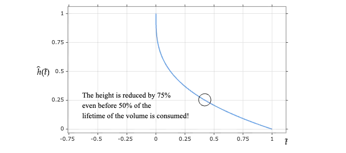
As you can see in the diagram, when the bottle seems to be empty, actually more than half of the liquid is still available.

Conclusions

Our suspicions were right: the level of the liquid decreases way faster at the beginning (look at that slope) than at the end.

Nevertheless, my girlfriend’s claim remains true: I do consume a lot of olive oil 😋

Looking back

Polya’s problem solving method is a great tool to solve problems because it reminds you to reflect about the way you solved the problem, to see if you can improve it or if you can learn something from it.

Hereby you find the adjustments I did to the path I followed to solve the problem originally, once it was solved.

Upper bound for the dimensionless time. When one looks at Equation (41), it is clear that the dimensionless time $\hat{t}$ is bounded by 1. Otherwise, the volume would be negative.

However, is this aligned with the dimensionless number that makes time dimensionless?

The dimensionless time $\hat{t}$ is defined as

$$\begin{equation} \hat{t} = t \cdot \frac{\dot{m}}{\Omega_0}. \end{equation}$$

Indeed, when one thinks about it, at a constant rate of pouring $\dot{m}$, the time it takes to empty the bottle is exactly equal to

$$\begin{equation} t_f = \frac{\Omega_0}{\dot{m}}. \end{equation}$$

Hence, since we have used the total time to empty the bottle to make time dimensionless, the dimensionless time $\hat{t}$ is bounded by 1,

$$\begin{equation} \hat{t} \in [0, 1]. \end{equation}$$

Decouple earlier. The first time I went through the equations I introduced the expression of the volume as a function of the height, Equation (9), in the mass conservation equation before identifying and solving the ODE. This was a mistake, because it made the algebraic operations messier.

When looking back at the whole, I realised it was simpler to solve the ODE for the volume first, Equation (32), and then replace the expression of the volume as a function of the height. This decoupled solving the ODE and the algebraic problem to find the expression of the height as a function of time.

In fact, up until this point the solution is general and valid for any bottle shape under the same boundary conditions.

To which stage does the definition of the boundary and initial conditions belong? While writing this document, I found it hard to decide in which section to talk about and mention the boundary and initial conditions for the mass conservation equation.

On the one hand, it could be argued that they belong to the “Understanding the problem” stage, because they are part of the problem’s details. On the other hand, they fitted naturally in the “Devising a plan” section, because their precise definition depends on the nature of the model equation we go for.

In my head, the model equations belong to the “Devising a plan” stage, because there can be multiple equations or approaches we could use to find the same unknown, e.g. empirical measurements, geometrical reasoning instead of the mass conservation equation, etc.

If you have an opinion on this matter, I would like to know about it.

Can I use the solution somewhere else?

This is one of my favorite questions from Polya’s book.

Imagine you have actually been instructed to solve not this problem, but the complete fluid mechanics problem of the liquid in the bottle.

At some point, you will need to plot the height as a function of time, for instance to compute the expected time to empty the bottle in days as a commercial feature. We can already use this simplified solution to get a good number, given some additional information about the bottle’s geometry and the pouring rate.

Or imagine that at some point in your complete fluid mechanics problem you need to use a numerical method to solve a more complex ODE.

This closed-form solution can be used as an initial condition for the numerical method; and it is assured to help it converge, since it captures the main features of the problem.

This is why I love addressing problems with a look for closed-form solutions, they are very informative about the stylized features of the problem, and they can be used for further, more detailed industrial applications.