A Beautiful Integral Hidden in a Bicycle • Adapting's Blog

Today, at the PyCon Spain (Vigo, Galicia), in the context of a ligthning talk, I presented the following problem from Classical Mechanics.

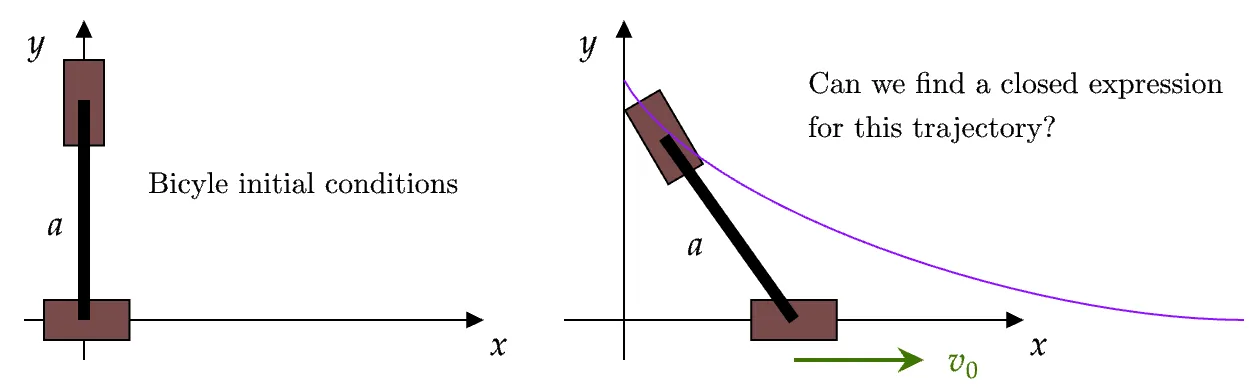
Given a bicycle whose front wheel is initially tilted 90 degrees, and moves forward at constant speed, can we find a closed expression for the trajectory of the rear wheel?

Let’s find out!

Strategy

To work out the trajectory of the rear wheel, we need to determine the angular velocity of the whole solid.

Because we know the speed of one point of our rigid body (the front wheel), we can work with the instantaneous center of rotation (ICR).

angular velocity = ICR + known linear velocity

The steps ahead are simple and clear. This is what we get from each of them and how we chain them.

Non-slip condition: the velocity vector of the rear tyre is aligned with the tyre itself;
Planar movement and ICR location: assuming the movement takes place in the plane (that is, the bike doesn’t tilt), we leverage the property that states:

the Instantaneous Center of Rotation (ICR) is the point where the normals to the velocity vectors of two separate points on a moving body intersect.

Relate angular velocity and linear velocity of the front tyre: this will give us a differential equation to compute the rotation angle.

Calculation of the angular motion

These are the triangles and heights involved in this problem.

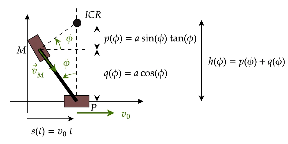
Two important remarks I want to highlight are: (1) the fact that the $\phi$ angle we have chosen is an angle that opens up from zero; (2) it is measured with respect to a line that, despite moving, does not rotate!

These details are paramount for the definition of angular velocity. We can work outside of them, but the math becomes a bit trickier.

The height $h(\phi)$ from the ICR to the front tyre is the sum of the two right sides of each triangle, $p(\phi)$ and $q(\phi)$ ,

\begin{align} h(\phi) &= p(\phi) + q(\phi), \\ h(\phi) &= a \sin{\left(\phi \right)} \tan{\left(\phi \right)} + a \cos{\left(\phi \right)}. \end{align}

Given $h(\phi)$ , we have a differential equation to find $\phi(t)$ :

\begin{align} h(\phi) \frac{d\phi}{dt} &= v_0, \\ \int \left(\sin{\left(\phi \right)} \tan{\left(\phi \right)} + \cos{\left(\phi \right)}\right) d\phi &= \frac{v_0}{a} t + C. \end{align}

With SymPy, we can obtain the primitive of this function:

\int \left(\sin{\left(\phi \right)} \tan{\left(\phi \right)} + \cos{\left(\phi \right)}\right) d\phi = \frac{1}{2}\ln{\left(\frac{\sin{\left(\phi \right)} + 1}{\sin{\left(\phi \right)} - 1} \right)}.

We are left with a final step, solving for $\phi(t)$ :

\begin{align} \frac{1}{2}\ln{\left(\frac{\sin{\left(\phi \right)} + 1}{\sin{\left(\phi \right)} - 1} \right)} &= \frac{v_0}{a}t, \\[5mm] \ldots \\[5mm] \phi(t) &= \sin^{-1}{\left(\tanh{\left(\frac{v_0}{a}t\right)} \right)}. \end{align}

Small detour to explain the hyperbolic tangent

Unless you are familiar with the primitive of the hyperbolic tangent, finding it in the expression for $\phi$ can be a surprise. It has do with the $1/2$ in front of the logarithm.

To see it clearly, let’s remove some notation noise and deal with a simplified equation,

\begin{align} \frac{1}{2}\ln{\left(\frac{u + 1}{u - 1} \right)} &= t, \\[3mm] \frac{u + 1}{u - 1} &= e^{2t}, \\[3mm] u &= \frac{e^{2t} - 1}{e^{2t} + 1}. \end{align}

This solution is already decent, but it gets better if we multiply and divide the numerator and denominator by $e^{-t}$ , to find the definition of the $\tanh$ ;

\begin{align} u &= \frac{e^{2t} - 1}{e^{2t} + 1} \cdot \frac{e^{-t}}{e^{-t}}, \\[3mm] u &= \frac{e^{t} - e^{-t}}{e^{t} + e^{-t}}, \\[3mm] u &= \tanh(t). \end{align}

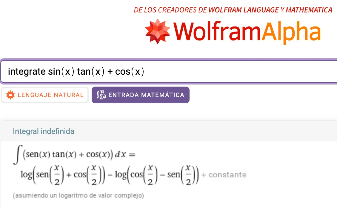
Comparison between WolframAlpha and Sympy

This talk was given in the context of the Pycon, so Python-based solutions were encouraged.

However, I tested the solution with another symbolic engine: WolframAlpha (web version). I was surprised to find out the solution was not as good. The result from WolframAlpha contains a more complex expression for the trigonometric functions inside the logarithm.

They are equivalent, of course, but this primitive requires further derivation steps.

Parametric equations of movement

Let’s get back to our original triangle, to find a parametric representation of our target trajectory.

Primitive equations

We can compute the location of the point M (rear wheel) by means of projections: we walk along lines of known length that lead to it, and as we walk, we project their length into each axis.

In this case, it means walking from the origin to the point P, and then going up the bicycle frame.

By doing so, we easily obtain the $x_M$ and $y_M$ expressions in terms of our degrees of freedom $t$ and $\phi$ (note that $s(t) = v_0 t$ ):

\begin{align} x_M &= v_0 t - a \sin(\phi), \\ y_M &= a \cos(\phi). \end{align}

Final parametric equations

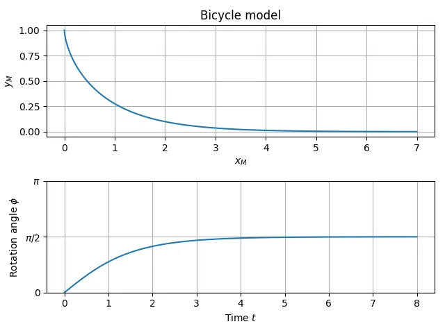
By plugging in our solution for $\phi(t)$ , we get a neat parametric representation of the location of the rear tyre,

\begin{align} \phi(t) &= \sin^{-1}{\left(\tanh{\left(\frac{v_0}{a}t\right)} \right)}, \\[2mm] x_M &= v_0 t - a \tanh(t), \\ y_M &= a \sqrt{1-\tanh^2(t)}. \end{align}

that we can plot and be satisfied about.

Location of the rear tyre and rotation angle.

Links

Repo with content: https://github.com/KikeM/pycones24-lightning-talk